Symbolic Algebra¶
Expressions and Operations¶
QNET includes a rich (and extensible) symbolic algebra system for quantum
mechanics and circuit models. The foundation of the symbolic algebra are the
Expression class and its subclass Operation.
A general algebraic expression has a tree structure. The branches of the tree
are operations; their children are the operands. The leaves of the tree are
scalars or “atomic” expressions, where “atomic” means not an object of type
Operation (e.g., a symbol)
For example, the KetPlus operation
defines the sum of Hilbert space vectors, represented as:
KetPlus(psi1, psi2, ..., psiN)
All operations follow this pattern:
Head(op1, op1, ..., opN)
where Head is a subclass of Operation and op1 .. opN are the
operands, which may be other operations, scalars, or atomic
Expression objects.
Note that all expressions (inluding operations) can have associated
arguments. For example KetSymbol takes label as an argument, and
the Hilbert space displacement operator Displace takes a
displacement amplitude as an argument. To avoid confusion between operands and
arguments, operations are required to take their operands as positional
arguments, and possible additional arguments as keyword arguments.
Expressions should generally not be instantiated directly, but through their
create() method allowing for simplifications. This is true
both for operations and atomic expressions. For example, instantiating
Displace with alpha=0 results in an IdentityOperator
(unlike direct instantiation, the create method of any class may or may not
return an instance of the same class). For operations, the create method
handles the application of algebraic rules such as associativity (translating
e.g. KetPlus(psi1, KetPlus(psi2, psi3)) into KetPlus(psi1, psi2, psi3))
Many operations are associated with infix operators, e.g.
a KetPlus instance is automatically
created if two instances of KetSymbol
are added with +. In this case, the create() method is used
automatically.
Expressions and Operations are considered immutable: any change to the expression tree (e.g. an algebraic simplification) generates a new expression.
Defining Operation subclasses¶
When extending an algebra with new operations, it is essential to define the
expression rewriting (“simplification”) rules that govern how new expressions
are instantiated. To this end, the _simplification class attribute of an
Expression subclass must be defined. This attribute contains a list
of callables. Each of these callables takes three parameters (the class, the
list args of positional arguments given to create() and
a dictionary kwargs of keyword arguments given to
create()) and return either a tuple of new args and
kwargs (which are then handed to the next callable), or an
Expression (which is directly returned as the result of the call to
Expression.create()).
Callables such as as assoc(), idem(), orderby(), and
filter_neutral() handle common algebraic properties such as associativity
or commutativity. The match_replace() and match_replace_binary()
callables are central to any more advanced simplification through pattern
matching. They delegate to a list of Patterns and replacements that are defined
in the _rules, respectively _binary_rules class attributes of the
Expression subclass.
The pattern matching rules may temporarily extended or modified using the
qnet.algebra.toolbox.core.extra_rules(),
qnet.algebra.toolbox.core.extra_binary_rules(), and
qnet.algebra.toolbox.core.no_rules() context managers.
Pattern matching¶
The application of patterns is central to symbolic algebra. Patterns are
defined and applied using the classed and helper routines in the
pattern_matching module.
There are two main places where pattern matching comes up:
- automatically, through
match_replace()andmatch_replace_binary()simplifications applied inside ofExpression.create(). - manually, through the
simplify()function (or theExpression.simplify()method)
Since inside match_replace() and
match_replace_binary(), patterns
are matched against expressions that are not yet instantiated (we call these
ProtoExpressions), the patterns in the _rules
and _binary_rules class attributes are always constructed using the
pattern_head() helper function. In contrast, patterns for
simplify() are usually created through the
pattern() helper function. The wc() function is used to associate
Expression arguments with wildcard names.
Algebraic Manipulations¶
While QNET automatically applies a large number of rules and simplifications if
expressions are instantiated through the create() method,
significant value is placed on manually manipulating algebraic expressions. In
fact, this is one of the design considerations that separates it from the
Sympy package: The rule-based transformations are both explicit and
optional, allowing to instantiate expressions exactly in the desired form, and
to apply specifc manipulations. Unlink in Sympy, the (tex) form of an
expressions will directly reflect the structure of the expression, and the
ordering of terms can be configured by the user. Thus, a
Jupyter Notebook could document a symbolic derivation in the exact form one
would normally write that derivation out by hand.
Common maniupulations and symbolic algorithms are collected in
qnet.algebra.toolbox.
Hilbert Space Algebra¶
The hilbert_space_algebra module defines a simple algebra
of finite dimensional or countably infinite dimensional Hilbert spaces.
Local/primitive degrees of freedom (e.g. a single multi-level atom or a cavity
mode) are described by a LocalSpace; it requires a label, and may
define a basis through the basis or dimension arguments. The LocalSpace
may also define custom identifiers for operators acting on that space
(subclasses of LocalOperator):
>>> a = Destroy(hs=1)
>>> ascii(a)
'a^(1)'
>>> hs1_custom = LocalSpace(1, local_identifiers={'Destroy': 'b'})
>>> b = Destroy(hs=hs1_custom)
>>> ascii(b)
'b^(1)'
Instances of LocalSpace combine via a product into
composite tensor product spaces are given by instances of the ProductSpace
Furthermore,
- the
TrivialSpacerepresents a trivial [1] Hilbert space \(\mathcal{H}_0 \simeq \mathbb{C}\) - the
FullSpacerepresents a Hilbert space that includes all possible degrees of freedom.
| [1] | trivial in the sense that \(\mathcal{H}_0 \simeq \mathbb{C}\), i.e., all states are multiples of each other and thus equivalent. |
Expressions in the operator, state, and superoperator algebra (discussed below)
will all be associated with a Hilbert space. If any expressions are intended to
be fed into a numerical simulation, all their associated Hilbert spaces must
have a known dimension. Since all expressions are immutable, it is important
to either define the all the LocalSpace instances they depend on with
basis or dimension arguments first, or to later generate new expression
with updated Hilbert spaces through the
substitute() routine.
Operator Algebra¶
The operator_algebra module implements and algebra of Hilbert space operators
Operator expressions are constructed from sums (OperatorPlus) and
products (OperatorTimes) of some basic elements, most importantly local
operators (subclasses of LocalOperator). This include some very common symbolic operator such as
- Harmonic oscillator mode operators \(a_s, a_s^\dagger\):
Destroy,Create - \(\sigma\)-switching operators \(\sigma_{jk}^s := \left| j \right\rangle_s \left \langle k \right|_s\):
LocalSigma - coherent displacement operators \(D_s(\alpha) := \exp{\left(\alpha a_s^\dagger - \alpha^* a_s\right)}\):
Displace - phase operators \(P_s(\phi) := \exp {\left(i\phi a_s^\dagger a_s\right)}\):
Phase - squeezing operators \(S_s(\eta) := \exp {\left[{1\over 2}\left({\eta {a_s^\dagger}^2 - \eta^* a_s^2}\right)\right]}\):
Squeeze
Furthermore, there exist symbolic representations for constants and symbols:
- the
IdentityOperator - the
ZeroOperator - an arbitrary
OperatorSymbol
There are also a number of algebraic operations that act only on a single operator as their only operand. These include:
- the Hilbert space
Adjointoperator \(X^\dagger\) PseudoInverseof operators \(X^+\) satisfying \(X X^+ X = X\) and \(X^+ X X^+ = X^+\) as well as \((X^+ X)^\dagger = X^+ X\) and \((X X^+)^\dagger = X X^+\)- the kernel projection operator (
NullSpaceProjector) \(\mathcal{P}_{{\rm Ker} X}\) satisfying both \(X \mathcal{P}_{{\rm Ker} X} = 0\) and \(X^+ X = 1 - \mathcal{P}_{{\rm Ker} X}\) - Partial traces over Operators \({\rm Tr}_s X\):
OperatorTrace
Examples¶
Say we want to write a function that constructs a typical Jaynes-Cummings Hamiltonian
for a given set of numerical parameters:
>>> from sympy import I
>>> def H_JC(Delta, Theta, epsilon, g):
...
...     # create Fock- and Atom local spaces
...     fock = LocalSpace('fock')
...     tls = LocalSpace('tls', basis=('e', 'g'))
...
...     # create representations of a and sigma
...     a = Destroy(hs=fock)
...     sigma = LocalSigma('g', 'e', hs=tls)
...
...     H = (Delta * sigma.dag() * sigma                    # detuning from atomic resonance
...         + Theta * a.dag() * a                           # detuning from cavity resonance
...         + I * g * (sigma * a.dag() - sigma.dag() * a)   # atom-mode coupling, I = sqrt(-1)
...         + I * epsilon * (a - a.dag()))                  # external driving amplitude
...     return H
Here we have allowed for a variable namespace which would come in handy if we wanted to construct an overall model that features multiple Jaynes-Cummings-type subsystems.
By using the support for symbolic sympy expressions as scalar pre-factors to operators, one can instantiate a Jaynes-Cummings Hamiltonian with symbolic parameters:
>>> Delta, Theta, epsilon, g = symbols('Delta, Theta, epsilon, g', real=True)
>>> H = H_JC(Delta, Theta, epsilon, g)
>>> H
ⅈ ε (-â^(fock)† + â⁽ᶠᵒᶜᵏ⁾) + Θ â^(fock)† â⁽ᶠᵒᶜᵏ⁾ + ⅈ g (â^(fock)† |g⟩⟨e|⁽ᵗˡˢ⁾ - â⁽ᶠᵒᶜᵏ⁾ |e⟩⟨g|⁽ᵗˡˢ⁾) + Δ |e⟩⟨e|⁽ᵗˡˢ⁾

>>> H.space
ℌ_fock ⊗ ℌ_tls
Operator products between commuting operators are automatically re-arranged such that they are ordered according to their Hilbert Space:
>>> Create(hs=2) * Create(hs=1)
â^(1)† â^(2)†
There are quite a few built-in replacement rules, e.g., mode operators products are normally ordered:
>>> Destroy(hs=1) * Create(hs=1)
𝟙 + â^(1)† â⁽¹⁾
Or for higher powers one can use the expand() method:
>>> (Destroy(hs=1) * Destroy(hs=1) * Destroy(hs=1) * Create(hs=1) * Create(hs=1) * Create(hs=1)).expand()
6 + â^(1)† â^(1)† â^(1)† â⁽¹⁾ â⁽¹⁾ â⁽¹⁾ + 9 â^(1)† â^(1)† â⁽¹⁾ â⁽¹⁾ + 18 â^(1)† â⁽¹⁾
State (Ket-) Algebra¶
The state_algebra module implements an algebra of Hilbert space states.
By default we represent states \(\psi\) as Ket vectors \(\psi \to | \psi \rangle\).
However, any state can also be represented in its adjoint Bra form, since those representations are dual:
States can be added to states of the same Hilbert space. They can be multiplied by:
- scalars, to just yield a rescaled state within the original space, resulting in
ScalarTimesKet - operators that act on some of the states degrees of freedom (but none that aren’t part of the state’s Hilbert space), resulting in a
OperatorTimesKet - other states that have a Hilbert space corresponding to a disjoint set of degrees of freedom, resulting in a
TensorKet
Furthermore,
And conversely,
- a
Bracan multiply aKetfrom the left to create a (partial) inner product objectBraKet. Currently, only full inner products are supported, i.e. theKetandBraoperands need to have the same space.
There are also the following symbolic states:
- arbitrary
KetSymbols - the
TrivialKetacting as the identity, and - the
ZeroKet.
Super-Operator Algebra¶
The super_operator_algebra contains an implementation of a
superoperator algebra, i.e., operators acting on Hilbert space operator or
elements of Liouville space (density matrices).
Each super-operator has an associated space property which gives the Hilbert space on which the operators the super-operator acts non-trivially are themselves acting non-trivially.
The most basic way to construct super-operators is by lifting ‘normal’ operators to linear pre- and post-multiplication super-operators:
>>> A, B, C = (OperatorSymbol(s, hs=FullSpace) for s in ("A", "B", "C"))
>>> SPre(A) * B
Â⁽ᵗᵒᵗᵃˡ⁾ B̂⁽ᵗᵒᵗᵃˡ⁾
>>> SPost(C) * B
B̂⁽ᵗᵒᵗᵃˡ⁾ Ĉ⁽ᵗᵒᵗᵃˡ⁾
>>> (SPre(A) * SPost(C)) * B
Â⁽ᵗᵒᵗᵃˡ⁾ B̂⁽ᵗᵒᵗᵃˡ⁾ Ĉ⁽ᵗᵒᵗᵃˡ⁾
>>> (SPre(A) - SPost(A)) * B        # Linear super-operator associated with A that maps B --> [A,B]
Â⁽ᵗᵒᵗᵃˡ⁾ B̂⁽ᵗᵒᵗᵃˡ⁾ - B̂⁽ᵗᵒᵗᵃˡ⁾ Â⁽ᵗᵒᵗᵃˡ⁾
The neutral elements of super-operator addition and multiplication are ZeroSuperOperator and IdentitySuperOperator, respectively.
Super operator objects can be added together in code via the infix ‘+’ operator and multiplied with the infix ‘*’ operator.
They can also be added to or multiplied by scalar objects.
In the first case, the scalar object is multiplied by the IdentitySuperOperator constant.
Super operators are applied to operators by multiplying an operator with superoperator from the left:
>>> S = SuperOperatorSymbol("S", hs=FullSpace)
>>> A = OperatorSymbol("A", hs=FullSpace)
>>> S * A
S⁽ᵗᵒᵗᵃˡ⁾[Â⁽ᵗᵒᵗᵃˡ⁾]
>>> isinstance(S*A, Operator)
True
The result is an operator.
Circuit Algebra¶
In their works on networks of open quantum systems [GoughJames08], [GoughJames09] Gough and James have introduced an algebraic method to derive the Quantum Markov model for a full network of cascaded quantum systems from the reduced Markov models of its constituents. This method is implemented in the circuit_algebra module.
A general system with an equal number \(n\) of input and output channels is described by the parameter triplet \(\left(\mathbf{S}, \mathbf{L}, H\right)\), where \(H\) is the effective internal Hamilton operator for the system, \(\mathbf{L} = (L_1, L_2, \dots, L_n)^T\) the coupling vector and \(\mathbf{S} = (S_{jk})_{j,k=1}^n\) is the scattering matrix (whose elements are themselves operators). An element \(L_k\) of the coupling vector is given by a system operator that describes the system’s coupling to the \(k\)-th input channel. Similarly, the elements \(S_{jk}\) of the scattering matrix are in general given by system operators describing the scattering between different field channels \(j\) and \(k\).
The only conditions on the parameters are that the hamilton operator is self-adjoint and the scattering matrix is unitary:
We adhere to the conventions used by Gough and James, i.e. we write the imaginary unit is given by \(i := \sqrt{-1}\), the adjoint of an operator \(A\) is given by \(A^*\), the element-wise adjoint of an operator matrix \(\mathbf{M}\) is given by \(\mathbf{M}^\sharp\). Its transpose is given by \(\mathbf{M}^T\) and the combination of these two operations, i.e. the adjoint operator matrix is given by \(\mathbf{M}^\dagger = (\mathbf{M}^T)^\sharp = (\mathbf{M}^\sharp)^T\).
The matrices of operators occuring in the SLH formalism are implemented in the matrix_algebra module.
Fundamental Circuit Operations¶
The basic operations of the Gough-James circuit algebra are given by:
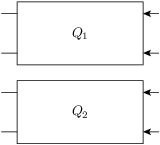
\(Q_1 \boxplus Q_2\)
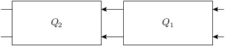
\(Q_2 \lhd Q_1\)
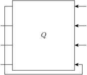
\([Q]_{1 \to 4}\)
In [GoughJames09], Gough and James have introduced two operations that allow the construction of quantum optical ‘feedforward’ networks:
- The concatenation product describes the situation where two arbitrary systems are formally attached to each other without optical scattering between the two systems’ in- and output channels
\[\begin{split}\left(\mathbf{S}_1, \mathbf{L}_1, H_1\right) \boxplus \left(\mathbf{S}_2, \mathbf{L}_2, H_2\right) = \left(\begin{pmatrix} \mathbf{S}_1 & 0 \\ 0 & \mathbf{S}_2 \end{pmatrix}, \begin{pmatrix}\mathbf{L}_1 \\ \mathbf{L}_1 \end{pmatrix}, H_1 + H_2 \right)\end{split}\]Note however, that even without optical scattering, the two subsystems may interact directly via shared quantum degrees of freedom.
- The series product is to be used for two systems \(Q_j = \left(\mathbf{S}_j, \mathbf{L}_j, H_j \right)\), \(j=1,2\) of equal channel number \(n\) where all output channels of \(Q_1\) are fed into the corresponding input channels of \(Q_2\)
\[\left(\mathbf{S}_2, \mathbf{L}_2, H_2 \right) \lhd \left( \mathbf{S}_1, \mathbf{L}_1, H_1 \right) = \left(\mathbf{S}_2 \mathbf{S}_1,\mathbf{L}_2 + \mathbf{S}_2\mathbf{L}_1 , H_1 + H_2 + \Im\left\{\mathbf{L}_2^\dagger \mathbf{S}_2 \mathbf{L}_1\right\}\right)\]
From their definition it can be seen that the results of applying both the series product and the concatenation product not only yield valid circuit component triplets that obey the constraints, but they are also associative operations.footnote{For the concatenation product this is immediately clear, for the series product in can be quickly verified by computing \((Q_1 \lhd Q_2) \lhd Q_3\) and \(Q_1 \lhd (Q_2 \lhd Q_3)\). To make the network operations complete in the sense that it can also be applied for situations with optical feedback, an additional rule is required: The feedback operation describes the case where the \(k\)-th output channel of a system with \(n\ge 2\) is fed back into the \(l\)-th input channel. The result is a component with \(n-1\) channels:
where the effective parameters are given by [GoughJames08]
Here we have written \(\mathbf{S}_{\cancel{[k,l]}}\) as a shorthand notation for the matrix \(\mathbf{S}\) with the \(k\)-th row and \(l\)-th column removed and similarly \(\mathbf{L}_{\cancel{[k]}}\) is the vector \(\mathbf{L}\) with its \(k\)-th entry removed. Moreover, it can be shown that in the case of multiple feedback loops, the result is independent of the order in which the feedback operation is applied. Note however that some care has to be taken with the indices of the feedback channels when permuting the feedback operation.
The possibility of treating the quantum circuits algebraically offers some valuable insights: A given full-system triplet \((\mathbf{S}, \mathbf{L}, H )\) may very well allow for different ways of decomposing it algebraically into networks of physically realistic subsystems. The algebraic treatment thus establishes a notion of dynamic equivalence between potentially very different physical setups. Given a certain number of fundamental building blocks such as beamsplitters, phases and cavities, from which we construct complex networks, we can investigate what kinds of composite systems can be realized. If we also take into account the adiabatic limit theorems for QSDEs (cite Bouten2008a,Bouten2008) the set of physically realizable systems is further expanded. Hence, the algebraic methods not only facilitate the analysis of quantum circuits, but ultimately they may very well lead to an understanding of how to construct a general system \((\mathbf{S}, \mathbf{L}, H)\) from some set of elementary systems. There already exist some investigations along these lines for the particular subclass of linear systems (cite Nurdin2009a,Nurdin2009b) which can be thought of as a networked collection of quantum harmonic oscillators.
Representation as Python objects¶
Python objects that are of the Circuit type have some of their operators overloaded to realize symbolic circuit algebra operations:
>>> A = CircuitSymbol('A', cdim=2)
>>> B = CircuitSymbol('B', cdim=2)
>>> print(srepr(A << B, cache={A: 'A', B: 'B'}))
SeriesProduct(A, B)
>>> print(srepr(A + B, cache={A: 'A', B: 'B'}))
Concatenation(A, B)
>>> print(srepr(FB(A, out_port=0, in_port=1), cache={A: 'A'}))
Feedback(A, out_port=0, in_port=1)
For a thorough treatment of the circuit expression simplification rules see Properties and Simplification of Circuit Algebraic Expressions.
Examples¶
Extending the JaynesCummings problem above to an open system by adding collapse operators \(L_1 = \sqrt{\kappa} a\) and \(L_2 = \sqrt{\gamma}\sigma.\)
>>> def SLH_JaynesCummings(Delta, Theta, epsilon, g, kappa, gamma, n=0):
...
...     # create Fock- and Atom local spaces
...     fock = LocalSpace('fock_%s' % n)
...     tls = LocalSpace('tls_%s' % n, basis=('e', 'g'))
...
...     # create representations of a and sigma
...     a = Destroy(hs=fock)
...     sigma = LocalSigma('g', 'e', hs=tls)
...
...     # Trivial scattering matrix
...     S = identity_matrix(2)
...
...     # Collapse/Jump operators
...     L1 = sqrt(kappa) * a                                    # Decay of cavity mode through mirror
...     L2 = sqrt(gamma) * sigma                                # Atomic decay due to spontaneous emission into outside modes.
...     L = Matrix([[L1], \
...                 [L2]])
...
...     # Hamilton operator
...     H = (Delta * sigma.dag() * sigma                        # detuning from atomic resonance
...         + Theta * a.dag() * a                               # detuning from cavity resonance
...         + I * g * (sigma * a.dag() - sigma.dag() * a)       # atom-mode coupling, I = sqrt(-1)
...         + I * epsilon * (a - a.dag()))                      # external driving amplitude
...
...     return SLH(S, L, H)
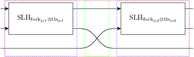
Consider now an example where we feed one Jaynes-Cummings system’s output into a second one:
>>> Delta, Theta, epsilon, g = symbols('Delta, Theta, epsilon, g', real=True)
>>> kappa, gamma = symbols('kappa, gamma')

>>> JC1 = SLH_JaynesCummings(Delta, Theta, epsilon, g, kappa, gamma, n=1)
>>> JC2 = SLH_JaynesCummings(Delta, Theta, epsilon, g, kappa, gamma, n=2)

>>> from qnet import circuit_identity as cid
>>> SYS = (JC2 + cid(1)) << CPermutation((0, 2, 1)) << (JC1 + cid(1))
The resulting system’s block diagram is:
and its overall SLH model is given by: