Symbolic Algebra
The Abstract Algebra module
The module features generic classes for encapsulating expressions and operations on expressions. It also includes some basic pattern matching and expression rewriting capabilities.
The most important classes to derive from for implementing a custom ‘algebra’ are qnet.algebra.abstract_algebra.Expression and qnet.algebra.abstract_algebra.Operation,
where the second is actually a subclass of the first.
The Operation class should be subclassed to implement any structured expression type
that can be specified in terms of a head and a (finite) sequence of operands:
Head(op1, op1, ..., opN)
An operation is assumed to have immutable operands, i.e., if one wishes to change the operands of an Operation,
one rather creates a new Operation with modified Operands.
Defining Operation subclasses
The single most important method of the Operation class is the qnet.algebra.abstract_algebra.Operation.create() classmethod.
Automatic expression rewriting by modifying/decorating the qnet.algebra.abstract_algebra.Operation.create() method
A list of class decorators:
qnet.algebra.abstract_algebra.assoc()qnet.algebra.abstract_algebra.idem()qnet.algebra.abstract_algebra.orderby()qnet.algebra.abstract_algebra.filter_neutral()qnet.algebra.abstract_algebra.check_signature()qnet.algebra.abstract_algebra.match_replace()qnet.algebra.abstract_algebra.match_replace_binary()
Pattern matching
The qnet.algebra.abstract_algebra.Wildcard class.
The qnet.algebra.abstract_algebra.match() function.
For a relatively simple example of how an algebra can be defined, see the Hilbert space algebra defined in qnet.algebra.hilbert_space_algebra.
Hilbert Space Algebra
This covers only finite dimensional or countably infinite dimensional Hilbert spaces.
The basic abstract class that features all properties of Hilbert space objects is given by: qnet.algebra.hilbert_space_algebra.HilbertSpace.
Its most important subclasses are:
- local/primitive degrees of freedom (e.g. a single multi-level atom or a cavity mode) are described by a
qnet.algebra.hilbert_space_algebra.LocalSpace. Every local space is identified by- composite tensor product spaces are given by instances of the
qnet.algebra.hilbert_space_algebra.ProductSpaceclass.- the
qnet.algebra.hilbert_space_algebra.TrivialSpacerepresents a trivial [1] Hilbert space \(\mathcal{H}_0 \simeq \mathbb{C}\)- the
qnet.algebra.hilbert_space_algebra.FullSpacerepresents a Hilbert space that includes all possible degrees of freedom.
| [1] | trivial in the sense that \(\mathcal{H}_0 \simeq \mathbb{C}\), i.e., all states are multiples of each other and thus equivalent. |
Examples
A single local space can be instantiated in several ways. It is most convenient to use the qnet.algebra.hilbert_space_algebra.local_space() method:
>>> local_space(1)
    LocalSpace(1, '')
This method also allows for the specification of the dimension of the local degree of freedom’s state space:
>>> s = local_space(1, dimension = 10)
>>> s
    LocalSpace(1, '')
>>> s.dimension
    10
>>> s.basis
    [0, 1, 2, 3, 4, 5, 6, 7, 8, 9]
Alternatively, one can pass a sequence of basis state labels instead of the dimension argument:
>>> lambda_atom_space = local_space('las', basis = ('e', 'h', 'g'))
>>> lambda_atom_space
    LocalSpace('las', '')
>>> lambda_atom_space.dimension
    3
>>> lambda_atom_space.basis
    ('e', 'h', 'g')
Finally, one can pass a namespace argument, which is useful if one is working with multiple copies of identical systems, e.g. if one instantiates multiple copies of a particular circuit component with internal degrees of freedom:
>>> s_q1 = local_space('s', namespace = 'q1', basis = ('g', 'h'))
>>> s_q2 = local_space('s', namespace = 'q2', basis = ('g', 'h'))
>>> s_q1
    LocalSpace('s', 'q1')
>>> s_q2
    LocalSpace('s', 'q2')
>>> s_q1 * s_q2
    ProductSpace(LocalSpace('s', 'q1'), LocalSpace('s', 'q2'))
The default namespace is the empty string ''.
Here, we have already seen the simplest way to create a tensor product of spaces:
>>> local_space(1) * local_space(2)
    ProductSpace(LocalSpace(1, ''), LocalSpace(2, ''))
Note that this tensor product is commutative
>>> local_space(2) * local_space(1)
    ProductSpace(LocalSpace(1, ''), LocalSpace(2, ''))
>>> local_space(2) * local_space(1) == local_space(1) * local_space(2)
    True
and associative
>>> (local_space(1) * local_space(2)) * local_space(3)
    ProductSpace(LocalSpace('1', ''), LocalSpace('2', ''), LocalSpace('3', ''))
The Operator Algebra module
This module features classes and functions to define and manipulate symbolic Operator expressions.
Operator expressions are constructed from sums (qnet.algebra.operator_algebra.OperatorPlus) and products (qnet.algebra.operator_algebra.OperatorTimes)
of some basic elements, most importantly local operators,
such as the annihilation (qnet.algebra.operator_algebra.Destroy) and creation (qnet.algebra.operator_algebra.Create) operators \(a_s, a_s^\dagger\)
of a quantum harmonic oscillator degree of freedom \(s\).
Further important elementary local operators are the switching operators
\(\sigma_{jk}^s := \left| j \right\rangle_s \left \langle k \right|_s\) (qnet.algebra.operator_algebra.LocalSigma).
Each operator has an associated qnet.algebra.operator_algebra.Operator.space property which gives the Hilbert space
(cf qnet.algebra.hilbert_space_algebra.HilbertSpace) on which it acts non-trivially.
We don’t explicitly distinguish between tensor-products \(X_s\otimes Y_r\) of operators on different degrees of freedom \(s,r\)
(which we designate as local spaces) and operator-composition-products \(X_s \cdot Y_s\) of operators acting on the same degree of freedom \(s\).
Conceptionally, we assume that each operator is always implicitly tensored with identity operators acting on all un-specified degrees of freedom.
This is typically done in the physics literature and only plays a role when tansforming to a numerical representation
of the problem for the purpose of simulation, diagonalization, etc.
All Operator classes
A complete list of all local operators is given below:
- Harmonic oscillator mode operators \(a_s, a_s^\dagger\) (cf
qnet.algebra.operator_algebra.Destroy,qnet.algebra.operator_algebra.Create)- \(\sigma\)-switching operators \(\sigma_{jk}^s := \left| j \right\rangle_s \left \langle k \right|_s\) (cf
qnet.algebra.operator_algebra.LocalSigma)- coherent displacement operators \(D_s(\alpha) := \exp{\left(\alpha a_s^\dagger - \alpha^* a_s\right)}\) (cf
qnet.algebra.operator_algebra.Displace)- phase operators \(P_s(\phi) := \exp {\left(i\phi a_s^\dagger a_s\right)}\) (cf
qnet.algebra.operator_algebra.Phase)- squeezing operators \(S_s(\eta) := \exp {\left[{1\over 2}\left({\eta {a_s^\dagger}^2 - \eta^* a_s^2}\right)\right]}\) (cf
qnet.algebra.operator_algebra.Squeeze)
Furthermore, there exist symbolic representations for constants and symbols:
- the identity operator (cf
qnet.algebra.operator_algebra.IdentityOperator)- and the zero operator (cf
qnet.algebra.operator_algebra.ZeroOperator)- an arbitrary operator symbol (cf
qnet.algebra.operator_algebra.OperatorSymbol)
Finally, we have the following Operator operations:
- sums of operators \(X_1 + X_2 + \dots + X_n\) (cf
qnet.algebra.operator_algebra.OperatorPlus)- products of operators \(X_1 X_2 \cdots X_n\) (cf
qnet.algebra.operator_algebra.OperatorTimes)- the Hilbert space adjoint operator \(X^\dagger\) (cf
qnet.algebra.operator_algebra.Adjoint)- scalar multiplication \(\lambda X\) (cf
qnet.algebra.operator_algebra.ScalarTimesOperator)
- pseudo-inverse of operators \(X^+\) satisfying \(X X^+ X = X\) and \(X^+ X X^+ = X^+\) as well
- as \((X^+ X)^\dagger = X^+ X\) and \((X X^+)^\dagger = X X^+\) (cf
qnet.algebra.operator_algebra.PseudoInverse)
- the kernel projection operator \(\mathcal{P}_{{\rm Ker} X}\) satisfying both \(X \mathcal{P}_{{\rm Ker} X} = 0\)
- and \(X^+ X = 1 - \mathcal{P}_{{\rm Ker} X}\) (cf
qnet.algebra.operator_algebra.NullSpaceProjector)- Partial traces over Operators \({\rm Tr}_s X\) (cf
qnet.algebra.operator_algebra.OperatorTrace)
For a list of all properties and methods of an operator object, see the documentation for the basic qnet.algebra.operator_algebra.Operator class.
Examples
Say we want to write a function that constructs a typical Jaynes-Cummings Hamiltonian
for a given set of numerical parameters:
def H_JaynesCummings(Delta, Theta, epsilon, g, namespace = ''):

    # create Fock- and Atom local spaces
    fock = local_space('fock', namespace = namespace)
    tls = local_space('tls', namespace = namespace, basis = ('e', 'g'))

    # create representations of a and sigma
    a = Destroy(fock)
    sigma = LocalSigma(tls, 'g', 'e')

    H = (Delta * sigma.dag() * sigma                        # detuning from atomic resonance
        + Theta * a.dag() * a                               # detuning from cavity resonance
        + I * g * (sigma * a.dag() - sigma.dag() * a)       # atom-mode coupling, I = sqrt(-1)
        + I * epsilon * (a - a.dag()))                      # external driving amplitude
    return H
Here we have allowed for a variable namespace which would come in handy if we wanted to construct an overall model that features multiple Jaynes-Cummings-type subsystems.
By using the support for symbolic sympy expressions as scalar pre-factors to operators, one can instantiate a Jaynes-Cummings Hamiltonian with symbolic parameters:
>>> Delta, Theta, epsilon, g = symbols('Delta, Theta, epsilon, g', real = True)
>>> H = H_JaynesCummings(Delta, Theta, epsilon, g)
>>> str(H)
    'Delta Pi_e^[tls] +  I*g ((a_fock)^* sigma_ge^[tls] - a_fock sigma_eg^[tls]) +  I*epsilon ( - (a_fock)^* + a_fock) +  Theta (a_fock)^* a_fock'
>>> H.space
    ProductSpace(LocalSpace('fock', ''), LocalSpace('tls', ''))
or equivalently, represented in latex via H.tex() this yields:
Operator products between commuting operators are automatically re-arranged such that they are ordered according to their Hilbert Space
>>> Create(2) * Create(1)
    OperatorTimes(Create(1), Create(2))
There are quite a few built-in replacement rules, e.g., mode operators products are normally ordered:
>>> Destroy(1) * Create(1)
    1 + Create(1) * Destroy(1)
Or for higher powers one can use the expand() method:
>>> (Destroy(1) * Destroy(1) * Destroy(1) * Create(1) * Create(1) * Create(1)).expand()
    (6 + Create(1) * Create(1) * Create(1) * Destroy(1) * Destroy(1) * Destroy(1) + 9 * Create(1) * Create(1) * Destroy(1) * Destroy(1) + 18 * Create(1) * Destroy(1))
The Circuit Algebra module
In their works on networks of open quantum systems [GoughJames08], [GoughJames09] Gough and James have introduced an algebraic method to derive the Quantum Markov model for a full network of cascaded quantum systems from the reduced Markov models of its constituents. A general system with an equal number \(n\) of input and output channels is described by the parameter triplet \(\left(\mathbf{S}, \mathbf{L}, H\right)\), where \(H\) is the effective internal Hamilton operator for the system, \(\mathbf{L} = (L_1, L_2, \dots, L_n)^T\) the coupling vector and \(\mathbf{S} = (S_{jk})_{j,k=1}^n\) is the scattering matrix (whose elements are themselves operators). An element \(L_k\) of the coupling vector is given by a system operator that describes the system’s coupling to the \(k\)-th input channel. Similarly, the elements \(S_{jk}\) of the scattering matrix are in general given by system operators describing the scattering between different field channels \(j\) and \(k\). The only conditions on the parameters are that the hamilton operator is self-adjoint and the scattering matrix is unitary:
We adhere to the conventions used by Gough and James, i.e. we write the imaginary unit is given by \(i := \sqrt{-1}\), the adjoint of an operator \(A\) is given by \(A^*\), the element-wise adjoint of an operator matrix \(\mathbf{M}\) is given by \(\mathbf{M}^\sharp\). Its transpose is given by \(\mathbf{M}^T\) and the combination of these two operations, i.e. the adjoint operator matrix is given by \(\mathbf{M}^\dagger = (\mathbf{M}^T)^\sharp = (\mathbf{M}^\sharp)^T\).
Fundamental Circuit Operations
The basic operations of the Gough-James circuit algebra are given by:
\(Q_1 \boxplus Q_2\)
\(Q_2 \lhd Q_1\)
\([Q]_{1 \to 4}\)
In [GoughJames09], Gough and James have introduced two operations that allow the construction of quantum optical ‘feedforward’ networks:
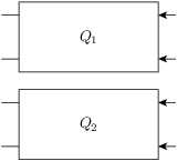
- The concatenation product describes the situation where two arbitrary systems are formally attached to each other without optical scattering between the two systems’ in- and output channels
\[\begin{split}\left(\mathbf{S}_1, \mathbf{L}_1, H_1\right) \boxplus \left(\mathbf{S}_2, \mathbf{L}_2, H_2\right) = \left(\begin{pmatrix} \mathbf{S}_1 & 0 \\ 0 & \mathbf{S}_2 \end{pmatrix}, \begin{pmatrix}\mathbf{L}_1 \\ \mathbf{L}_1 \end{pmatrix}, H_1 + H_2 \right)\end{split}\]Note however, that even without optical scattering, the two subsystems may interact directly via shared quantum degrees of freedom.
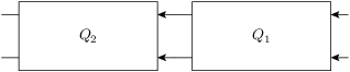
- The series product is to be used for two systems \(Q_j = \left(\mathbf{S}_j, \mathbf{L}_j, H_j \right)\), \(j=1,2\) of equal channel number \(n\) where all output channels of \(Q_1\) are fed into the corresponding input channels of \(Q_2\)
\[\left(\mathbf{S}_2, \mathbf{L}_2, H_2 \right) \lhd \left( \mathbf{S}_1, \mathbf{L}_1, H_1 \right) = \left(\mathbf{S}_2 \mathbf{S}_1,\mathbf{L}_2 + \mathbf{S}_2\mathbf{L}_1 , H_1 + H_2 + \Im\left\{\mathbf{L}_2^\dagger \mathbf{S}_2 \mathbf{L}_1\right\}\right)\]
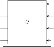
From their definition it can be seen that the results of applying both the series product and the concatenation product not only yield valid circuit component triplets that obey the constraints, but they are also associative operations.footnote{For the concatenation product this is immediately clear, for the series product in can be quickly verified by computing \((Q_1 \lhd Q_2) \lhd Q_3\) and \(Q_1 \lhd (Q_2 \lhd Q_3)\). To make the network operations complete in the sense that it can also be applied for situations with optical feedback, an additional rule is required: The feedback operation describes the case where the \(k\)-th output channel of a system with \(n\ge 2\) is fed back into the \(l\)-th input channel. The result is a component with \(n-1\) channels:
where the effective parameters are given by [GoughJames08]
Here we have written \(\mathbf{S}_{\cancel{[k,l]}}\) as a shorthand notation for the matrix \(\mathbf{S}\) with the \(k\)-th row and \(l\)-th column removed and similarly \(\mathbf{L}_{\cancel{[k]}}\) is the vector \(\mathbf{L}\) with its \(k\)-th entry removed. Moreover, it can be shown that in the case of multiple feedback loops, the result is independent of the order in which the feedback operation is applied. Note however that some care has to be taken with the indices of the feedback channels when permuting the feedback operation.
The possibility of treating the quantum circuits algebraically offers some valuable insights: A given full-system triplet \((\mathbf{S}, \mathbf{L}, H )\) may very well allow for different ways of decomposing it algebraically into networks of physically realistic subsystems. The algebraic treatment thus establishes a notion of dynamic equivalence between potentially very different physical setups. Given a certain number of fundamental building blocks such as beamsplitters, phases and cavities, from which we construct complex networks, we can investigate what kinds of composite systems can be realized. If we also take into account the adiabatic limit theorems for QSDEs (cite Bouten2008a,Bouten2008) the set of physically realizable systems is further expanded. Hence, the algebraic methods not only facilitate the analysis of quantum circuits, but ultimately they may very well lead to an understanding of how to construct a general system \((\mathbf{S}, \mathbf{L}, H)\) from some set of elementary systems. There already exist some investigations along these lines for the particular subclass of linear systems (cite Nurdin2009a,Nurdin2009b) which can be thought of as a networked collection of quantum harmonic oscillators.
Representation as Python objects
This file features an implementation of the Gough-James circuit algebra rules as introduced in [GoughJames08] and [GoughJames09].
Python objects that are of the qnet.algebra.circuit_algebra.Circuit type have some of their operators overloaded to realize symbolic circuit algebra operations:
>>> A = CircuitSymbol('A', 2)
>>> B = CircuitSymbol('B', 2)
>>> A << B
    SeriesProduct(A, B)
>>> A + B
    Concatenation(A, B)
>>> FB(A, 0, 1)
    Feedback(A, 0, 1)
For a thorough treatment of the circuit expression simplification rules see Properties and Simplification of Circuit Algebraic Expressions.
Examples
Extending the JaynesCummings problem above to an open system by adding collapse operators \(L_1 = \sqrt{\kappa} a\) and \(L_2 = \sqrt{\gamma}\sigma.\)
def SLH_JaynesCummings(Delta, Theta, epsilon, g, kappa, gamma, namespace = ''):

    # create Fock- and Atom local spaces
    fock = local_space('fock', namespace = namespace)
    tls = local_space('tls', namespace = namespace, basis = ('e', 'g'))

    # create representations of a and sigma
    a = Destroy(fock)
    sigma = LocalSigma(tls, 'g', 'e')

    # Trivial scattering matrix
    S = identity_matrix(2)

    # Collapse/Jump operators
    L1 = sqrt(kappa) * a                                    # Decay of cavity mode through mirror
    L2 = sqrt(gamma) * sigma                                # Atomic decay due to spontaneous emission into outside modes.
    L = Matrix([[L1], \
                [L2]])

    # Hamilton operator
    H = (Delta * sigma.dag() * sigma                        # detuning from atomic resonance
        + Theta * a.dag() * a                               # detuning from cavity resonance
        + I * g * (sigma * a.dag() - sigma.dag() * a)       # atom-mode coupling, I = sqrt(-1)
        + I * epsilon * (a - a.dag()))                      # external driving amplitude

    return SLH(S, L, H)
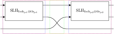
Consider now an example where we feed one Jaynes-Cummings system’s output into a second one:
Delta, Theta, epsilon, g = symbols('Delta, Theta, epsilon, g', real = True)
kappa, gamma = symbols('kappa, gamma')

JC1 = SLH_JaynesCummings(Delta, Theta, epsilon, g, kappa, gamma, namespace = 'jc1')
JC2 = SLH_JaynesCummings(Delta, Theta, epsilon, g, kappa, gamma, namespace = 'jc2')

SYS = (JC2 + cid(1)) << P_sigma(0, 2, 1) << (JC1 + cid(1))
The resulting system’s block diagram is:
and its overall SLH model is given by:
The Super-Operator Algebra module
The specification of a quantum mechanics symbolic super-operator algebra. Each super-operator has an associated space property which gives the Hilbert space on which the operators the super-operator acts non-trivially are themselves acting non-trivially.
The most basic way to construct super-operators is by lifting ‘normal’ operators to linear pre- and post-multiplication super-operators:
>>> A, B, C = OperatorSymbol("A", FullSpace), OperatorSymbol("B", FullSpace), OperatorSymbol("C", FullSpace)
>>> SPre(A) * B
    A * B
>>> SPost(C) * B
    B * C
>>> (SPre(A) * SPost(C)) * B
    A * B * C
>>> (SPre(A) - SPost(A)) * B        # Linear super-operator associated with A that maps B --> [A,B]
    A * B - B * A
There exist some useful constants to specify neutral elements of super-operator addition and multiplication:
ZeroSuperOperatorIdentitySuperOperator
Super operator objects can be added together in code via the infix ‘+’ operator and multiplied with the infix ‘*’ operator. They can also be added to or multiplied by scalar objects. In the first case, the scalar object is multiplied by the IdentitySuperOperator constant.
Super operators are applied to operators by multiplying an operator with superoperator from the left:
>>> S = SuperOperatorSymbol("S", FullSpace)
>>> A = OperatorSymbol("A", FullSpace)
>>> S * A
    SuperOperatorTimesOperator(S, A)
>>> isinstance(S*A, Operator)
    True
The result is an operator.
The State (Ket-) Algebra module
This module implements a basic Hilbert space state algebra where by default we represent states \(\psi\) as ‘Ket’ vectors \(\psi \to | \psi \rangle\). However, any state can also be represented in its adjoint Bra form, since those representations are dual:
States can be added to states of the same Hilbert space. They can be multiplied by:
- scalars, to just yield a rescaled state within the original space
- operators that act on some of the states degrees of freedom (but none that aren’t part of the state’s Hilbert space)
- other states that have a Hilbert space corresponding to a disjoint set of degrees of freedom
Furthermore,
- a
Ketobject can multiply aBraof the same space from the left to yield aKetBratype operator.
And conversely,
- a
Bracan multiply aKetfrom the left to create a (partial) inner product objectBraKet. Currently, only full inner products are supported, i.e. theKetandBraoperands need to have the same space.